

Introduction
Atmospheric predictability relies heavily on the accuracy of initial conditions. Small errors in these initial conditions can grow rapidly over time, amplified by the atmosphere’s nonlinear and chaotic nature. Sensitivity analyses are a crucial tool, letting researchers examine how a specific forecast metric or variable, such as precipitation over a particular region, responds to minute changes in the atmospheric patterns found upstream at the start of the forecast (the gradient ∂K/∂Xi). These studies are valuable for things like targeted observing, designing observing networks, parameter estimation, and data assimilation.
Sensitivities reveal the interconnectedness of atmospheric variables across space and time, and can potentially uncover the physical processes driving forecast evolution. This study explores the latter area using a new generation of Artificial Intelligence (AI) data-driven weather models to investigate the physical validity of relationships learned by the AI.
AI data-driven models are transforming weather forecasting, providing forecast skill that’s competitive with state-of-the-art dynamical (physics-based) models, but at a much lower computational cost (after training). These models are built on neural networks, which combine differentiable linear operators and nonlinear activation functions. They are optimized using the backpropagation algorithm, supported by modern libraries via auto-differentiation. The backpropagation algorithm, with its associated libraries, facilitates the computation of gradients (sensitivity fields) by applying the “chain rule.” This process effectively traces information backward from the output layer (the target variable of interest) to the input layer (the initial conditions). This can be done in a matter of minutes with a single CPU, or even seconds on a GPU.
These properties make AI models attractive for initial condition sensitivity studies and can avoid limitations in dynamical models, which often rely on the adjoint of a linearized version of the model. This method linearizes the evolution of perturbations along the initial trajectory, which restricts its use to forecast lead times of only a few days. Furthermore, the formulation of the adjoint model is complex, especially with process-based parameterizations, and it requires running the nonlinear dynamical model. This, in turn, increases the computational burden of the methodology. Sensitivities derived from AI data-driven models, on the other hand, are not restricted by linearity assumptions. They are also simpler to compute. For example, the predictability limit of the 2021 Pacific Northwest heatwave was analyzed using backpropagation to examine forecast error at weather and sub-seasonal timescales.
This study examines how well an AI-driven data model can replicate the sensitivities of Cyclone Xynthia, using values from the adjoint of a physics-based model as a benchmark. This comparison aims to determine whether AI models are drawing on information from physically realistic relationships to generate forecasts as well as gauge the usefulness of these models as initial condition sensitivity tools.
Results
Case Study: Cyclone Xynthia
Strong winds and heavy precipitation from mid-latitude cyclones have significant socio-economic effects that make them very important to study. Understanding the dynamics behind these events and improving forecast accuracy are essential to society. Climate change simulations also predict increases in the intensity and frequency of precipitation extremes linked to extratropical cyclones under future emission scenarios compared to pre-industrial conditions. Cyclones are complex phenomena, often driven by nonlinear interactions among dynamic and thermodynamic processes. In the current context, Cyclone Xynthia is being presented as a case study to offer insight into the potential of AI-driven models for sensitivity analysis while also evaluating the physical realism of the relationships these models highlight.
Cyclone Xynthia was a high-impact event that led to significant socio-economic damage in Western Europe. It caused high winds, extreme precipitation, flooding, and large ocean waves, which led to over 50 deaths across several European countries. Cyclone Xynthia began on February 26th over a low-pressure center south of the Azores Islands (996 hPa), on the edge of an atmospheric river (AR). Atmospheric rivers are elongated structures in the atmosphere that transport moisture from the tropics to mid-latitudes, often associated with extreme precipitation. This particular atmospheric river extended roughly 6,500 km from the southwest to the northeast, from the Azores to Southern Iberia, with an average width of approximately 700 km and carrying up to 30 kg of water vapor per meter square.
The system quickly intensified as it passed over the coasts of Portugal and Northern Spain. It then reached Western France on February 28th with winds exceeding 30 m/s, waves reaching 7.5 m, and rainfall nearly 2 m. After March 1st, the severity of the event diminished as it moved inland towards Central Europe. The evolution of Cyclone Xynthia is illustrated in Figure 1, and additional details can found in the reference material.

Figure 1: Evolution of cyclone Xynthia.
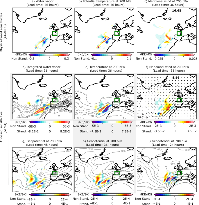
Figure 2: Comparison of physics-based and AI-based sensitivity fields for cyclone Xynthia.
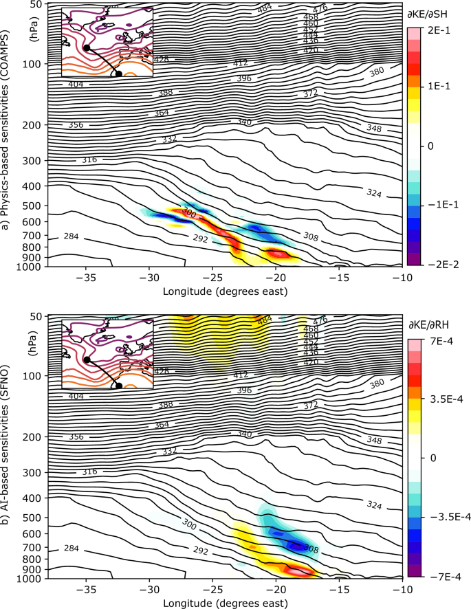
Figure 3: Vertical cross-section of the sensitivity fields of kinetic energy over the Bay of Biscay for cyclone Xynthia.
A sensitivity analysis of Cyclone Xynthia was carried out using a dynamical and adjoint model. The purpose of this analysis was to investigate the factors influencing the predictability of this extreme weather event. In this study, sensitivity fields of kinetic energy (KE) over the Bay of Biscay were computed for a 36-hour forecast, using the initial conditions from February 26th at 12 UTC. These fields were obtained through the Coupled Ocean-Atmosphere Mesoscale Prediction System (COAMPS) adjoint model, which uses a non-hydrostatic dynamical core. The model was implemented over a nested domain with a 45-km horizontal grid spacing for the coarse mesh and 15-km spacing for the fine mesh. The model also included a microphysics parameterization for cloud water, rainwater, snow, and graupel concentrations. A subgrid-scale parameterization for deep convection was also integrated. The sensitivities from the original study are replotted here to allow for a closer comparison with the AI-based results.
There are differences in how sensitivities are computed between the AI and the original study’s approaches, so the comparison presented is qualitative. First, the AI model is initialized using the European Centre for Medium-Range Weather Forecasts Reanalysis version 5 (ERA5) data for its initial condition sensitivities. The COAMPS model, on the other hand, is initialized from the National Oceanic and Atmospheric Administration (NOAA) Global Forecast System (GFS). Second, the range of variables simulated differs between the two models. Therefore, AI-based sensitivities are being compared using the closest available proxies in COAMPS. For example, relative humidity from the AI model is compared to the specific humidity in COAMPS, as shown in Figure 3. Third, vertical and spatial resolutions also vary between these two models. COAMPS uses z-sigma vertical levels, a grid mesh of 45 km for the coarse mesh, and a 15 km mesh for the fine mesh horizontal grid increments, whereas the AI model simulates variables at 13 pressure levels on a 0.25° latitude-longitude grid. Fourth, the method for calculating kinetic energy shows a slight difference. While D14 includes the vertical wind component, the AI model only considers the zonal and meridional components.
All of these factors must be considered when analyzing the results in the following sections.
Forecasting Cyclone Xynthia
Figure 1 shows the evolution of Cyclone Xynthia as represented by ERA5 and as predicted by the Spherical Fourier Neural Operator (SFNO). The SFNO predicts a rapid intensification of Xynthia, with winds carrying kinetic energy approaching 200 m2/s2. The low-pressure system is predicted to move towards the coast of Portugal by February 27th at 12 UTC, which matches ERA5. By February 28th at 00 UTC, Cyclone Xynthia reached the Bay of Biscay and the western coast of France. The SFNO accurately captures the strong pressure gradient in this region and predicts slightly less kinetic energy than ERA5, which still surpasses values of 200 m2/s2 in the region. A comparison between SFNO and the Integrated Forecasting System (IFS)—ECMWF’s state-of-the-art dynamical prediction model—shows similar values of root mean squared error between models, with 58 and 82 m2/s2, respectively, for the kinetic energy at the 36-h forecast time. These values were averaged over the Bay of Biscay on February 28th at 00 UTC. ERA5 was used as the ground truth. The IFS forecast was initialized using its analysis dataset, which may also explain why the IFS had a slightly greater RMSE than SFNO when validated against ERA5.
Initial Condition Sensitivities
Figure 2 displays the sensitivity fields of kinetic energy (KE) over the Bay of Biscay for a 36-hour forecast lead time, with the initial condition set to 12 UTC on February 26th. Specifically, the 45-km physics-based sensitivities for water vapor, 700-hPa potential temperature, and 700-hPa meridional wind from the initial study are compared with the AI-based sensitivities for integrated water vapor, 700-hPa air temperature, and 700-hPa meridional wind. The 700 hPa level was chosen because it played a prominent role during Cyclone Xynthia. The color scales for each variable are different to improve the visualizations. The AI-based maps have two color scales: one for sensitivities computed relative to the standardized version of the inputs and one for sensitivities computed relative to the non-standardized version of the inputs. These scales allow for a direct comparison with physics-based sensitivities, with comparisons among AI sensitivities, indicating each variable’s relative importance to the KE. Positive values (red) indicate areas where initial condition increases lead to an increase in KE at the final time. Negative values (blue) indicate initial condition decreases resulting in a final-time increase in KE.
The results reveal that a small moisture filament, approximately 40 km wide, within the atmospheric river is the main contributor to cyclone development. This filament extends west of the Azores, in a southwest-northeast direction toward the coast of Portugal, with the greatest sensitivity values between the 500 and 1000 hPa levels (Fig. 3a). Temperature sensitivities align with this moisture filament (Fig. 2b), while wind sensitivities are concentrated in short-wave troughs over the central and North Atlantic. This suggests that stronger southerly winds at the initial time lead to increased kinetic energy at the final time (Fig. 2c). Negative water vapor sensitivities flank the positive moisture filament inside the AR, indicating that an intensification of the winds occurs from increasing moisture gradient in this region (Fig. 2a).
The AI-based and physics-based sensitivities are remarkably similar, showing nearly identical spatial structures for the examined variables. The S-shaped sensitivity structure west of the coast of Portugal along the short-wave trough, which is present in the meridional wind, is well-captured by the AI model (Fig. 2f). Both the integrated water vapor and temperature fields also show elongated structures along the AR. However, although the AI-based model’s maximum sensitivity values are generally lower than the physics-based model’s, the aggregated sensitivities across the map are of a similar magnitude. This can be attributed to the non-zero influence of non-relevant features caused by complex interactions within the neural network. Even though the AI-based model has a higher-resolution grid, its sensitivities appear coarser than those of the physics-based model. This is likely because the effective resolution of AI models is known to be lower than the original resolution used during the model training.
The AI-based sensitivities for geopotential are also shown (Fig. 2g–i), and they are notably more pronounced than those of the other variables. These sensitivities exhibit wave-like patterns, which may result from the projection of sensitivities onto a Rossby wave packet in the waveguide, based on experience from adjoint sensitivity studies. This packet interacts with precipitation and diabatic processes, propagating downstream. As the lead time increases from 24 to 48 h, these wave-like patterns shift westward, moving further offshore and upstream of the response function. This shift is consistent with the expected eastward propagation over time, driven by background westerly winds and highlights the physical consistency of the relationships learned by the AI model.
Figure 3b demonstrates the relative humidity (RH) sensitivities in a vertical cross-section connecting two locations in the northwest-southeast direction, crossing the AR. The positions of these two locations were based on the sensitivity maximums shown in Fig. 2. These same locations are used to plot the specific humidity (SH) sensitivities from the physics-based model in D14 (Fig. 3a). As in Fig. 2, the comparison between the approaches is qualitative, since SFNO (COAMPS) does not include SH (or RH) in its variable set. The x-axis presents the longitudes between these two locations, and the y-axis corresponds to pressure levels. The areas of maximum sensitivity are found between longitudes -25° and -15°, spanning from the surface to 450 hPa. The positive-negative dipole indicates that an increased moisture gradient within the AR at the initial time leads to an increase in kinetic energy over the Bay of Biscay at the final time, also tilting against the sloping warm frontal zone. Overall, the vertical sensitivities are aligned well with the physics-based fields, and only minor differences exist in the positions of the maximum values. These differences might be explained by the fundamental differences between the two models, which include distinct horizontal and vertical resolutions as well as methodological differences in how predictions are generated.
A positive sensitivity is observed at the upper levels of the atmosphere, the relationship suggesting spurious or noisy correlations learned by the AI model. This is notable because, to the best of our knowledge, no physical principle supports this relationship between upper-level atmospheric conditions and low-level final-time kinetic energy. Identifying these non-physical links is essential in AI-based weather modeling, since it could help guide the development of more reliable and physically consistent models in the future.
Evolution of Sensitivity-Based Perturbations
Sensitivity-based perturbations, scaled to align with estimates of initial condition uncertainty, are applied to the variables at the initial time. Figure 4 shows the difference between the perturbed and the control forecasts for the kinetic energy at 12, 24, and 36 h of forecast lead time.
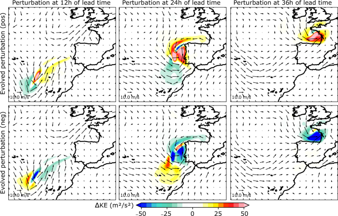
Figure 4: Evolved perturbation fields for the kinetic energy at 12, 24 and 36 h of lead time.
Two perturbed forecasts were generated. The first added a sensitivity-based perturbation to the initial condition (positive perturbation, first row). The other one changed the sign (negative perturbation, second row). The evolved kinetic energy perturbations grow in intensity from approximately 5–25 m2/s2 at 12 h of forecast lead time to 15–50 m2/s2, and they follow the path of the low-pressure system at each forecast lead time until it reaches the Bay of Biscay on February 28th at 00 UTC. The positive perturbations, which added moisture to the initial condition and, in turn, increased the moisture and temperature gradients along the AR, simulate an intensification of the winds associated with Xynthia. Negative perturbations, on the other hand, create the opposite response, overall reducing the kinetic energy of Xynthia compared to the control forecast. These are expected results, since the perturbation fields were built based on the sensitivity fields. The symmetry between positive and negative perturbations at final time is evidence of quasi-linear perturbation growth over this time period, which can also be seen in the original study.
Figure 5 presents, over the Bay of Biscay, the control and perturbed AI forecasts at the 36-h forecast time, showing the predicted values for the kinetic energy, in color, and the mean sea level pressure, in contours.
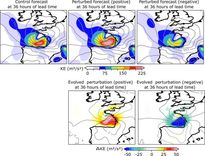
Figure 5: Control and perturbed forecasts, and evolved perturbations of kinetic energy for cyclone Xynthia at 36 h of lead time.
The forecast shows a low-level jet in the southern area of the low pressure, from the west coast of Spain to the west coast of France. The positive and negative perturbed forecasts increase and decrease the kinetic energy in the region, reaching maxima of 70 and –70 m2/s2, respectively, while also modifying the low-pressure system. These results are similar to the ones shown in the original study and show similar spatial structures. Differences in the mean sea level pressure between the perturbed and control forecasts are represented by contours in Fig. 5 every 1 hPa, showing a north-to-south gradient, with the evolved perturbation fields consistent with the results from the dynamical model. However, the change in pressure is smaller than in the original study.
Discussion
AI models are being examined as initial-condition sensitivity tools that explore links learned between various fields as the forecast evolves. This provides a mechanism to assess the physical realism of AI models, which is something that hasn’t been explored to any great degree. So far, these models have produced consistent responses to simple dynamical tests but have presented error-growth patterns from small-amplitude initial condition perturbations that did not reflect the characteristic “butterfly” effect of dynamical models. Here, sensitivities from the Spherical Fourier Neural Operator (SFNO) AI model are compared to those from a dynamical model, which are used as references for identifying physically plausible links in the atmosphere. The chosen case study is Cyclone Xynthia, a high-impact extreme weather event in Western Europe in 2010, whose sensitivity fields had previously been examined by way of dynamical and adjoint models.
The SFNO shows high sensitivities for integrated water vapor is consistent with the results from the original study and other studies where moisture was identified as a key driver for cyclone development. Moreover, SFNO moisture sensitivity maximums are located over a warm filament of air within an atmospheric river, just like the original study. For variables like temperature and meridional wind velocity, the spatial structures between the AI and dynamical models are comparable. Vertical sensitivities are remarkably similar for relative humidity as well. Sensitivity-based perturbations simulate higher values of kinetic energy over The Bay of Biscay, similar to the results of the original study.
The AI data-driven model was robust under a series of simple physical tests, such as shifting the perturbation fields 20° west or 20° west and 25° north across areas of low sensitivity. It showed little-to-no differences in the forecasts compared to the control forecast (not shown). Also, the evolved kinetic energy perturbations followed the path of the low-pressure system, showing no changes elsewhere in the domain. The sensitivities amplify and grow with an increased forecast lead time and exhibit wave structures, which also frequently appear in the fields from adjoint models.
Unlike dynamical models, the SFNO exhibits a strong dependence on geopotential. This can mask the influence of other variables. That might imply a lack of consistent inter-variable links in the model, as the evolved perturbation fields’ behavior demonstrates, where the sea-level pressure did not show a change as large as in the original study under moisture-based-perturbation simulations. This strong dependence on geopotential has been confirmed by conducting similar experiments in other cyclones and was also identified in other deep learning models for statistical applications. There this behavior was attributed to the potential co-variabilities in the model within the set of explanatory variables.
The aforementioned properties demonstrate the potential of AI data-driven models to learn physical relationships to some degree and their ability to automatically identify links between atmospheric variables over space and time. While fully consistent and complex physical relationships still require improvements, these models are already able to capture important relationships between atmospheric variables, and produce accurate forecasts based on them. That is, the general sensitivity characteristics are not model/technique dependent (although the specific details do vary with model). Obtaining similar results through differing modeling approaches—the adjoint of a physical model and an AI model—supports the robustness and generality of the results. This study clearly demonstrates the potential of these tools for sensitivity studies, especially given the rapid computation of the gradients. The overall properties of neural networks and the backpropagation algorithm can also enable sensitivity studies at longer timescales, since they’re unconstrained by linear assumptions in the same way the adjoint model is. This will be explored in future work.
Methods
AI Data-Driven Model: Spherical Fourier Neural Operator (SFNO)
The Spherical Fourier Neural Operator (SFNO) is an AI data-driven model designed to forecast the next 6 h of weather at 0.25° of spatial resolution, given the same set of variables at the initial time. Forecasts at longer lead times can be produced by using the model outputs as inputs to the next iteration. SFNO is an updated version of Fourcastnet, which built on the Adaptive Fourier Neural Operator (AFNO) to perform the Fast Fourier Transform (FFT) with a Vision Transformer backbone. It takes advantage of the benefits of self-attention to extract meaningful patterns from spatial data. This model configuration pioneered the use of AI data-driven models for weather forecasting, being the first to achieve forecast skill on par with the Integrated Forecasting System (IFS)—followed by Graphical Neural Networks-based topologies (GraphCast and AIFS) or other transformer-based ones (FuXi and Pangu-Weather). SFNO builds on spherical harmonics, in contrast to AFNO’s FFT.
The trained model can be accessed at the ECMWF AI-models github: https://github.com/ecmwf-lab/ai-models. Once trained, 36-h forecasts for Cyclone Xynthia were produced in the order of minutes using a single CPU. Significantly faster times (on the order of seconds) could be achieved using GPUs.
Computation of Initial Condition Sensitivities with AI Data-Driven Models
To compute the sensitivity of the kinetic energy (KE) over the Bay of Biscay at the final time, relative to the variables at the initial time, five steps are followed. The process is outlined below:
-
Standardization of input variables: The input variables are first standardized using the training data’s mean and standard deviation. A complete list of the input variables is shown in the “Data” section.
-
Model forecasting: The AI data-driven model’s auto-regression mechanism is then unfolded. The model is iterated six times to generate a 36-h forecast, and the outputs of each step are used as inputs for the next step.
-
De-standardization of prediction: The prediction is de-standardized by applying the training mean and standard deviation, which returns the results to the original scale of the variables.
-
Kinetic energy calculation: Kinetic energy is calculated by summing the squares of the predicted zonal (u) and meridional (v) wind components at each grid point within the Bay of Biscay – the result is then averaged over the total number of grid points. The formula for the kinetic energy is as follows:
KE = 0.5 * Σi (ui^2 + vi^2) / N -
Sensitivity computation: Finally, the gradients—i.e., the partial derivatives of KE with respect to the input variables at the initial time—are calculated using the chain rule and the backpropagation algorithm from PyTorch’s automatic differentiation package. The chain rule for sensitivity computation is presented in Equation 1. This step’s calculations are conceptually similar to the gradient calculations used during model training for gradient descent.
The sensitivity fields were computed within minutes using a single CPU, with significantly faster times (seconds) being achieved using GPUs.
∂KE/∂X = (∂KE/∂Y) * (∂Y/∂F6) * (∂F6/∂F5) * ... * (∂F1/∂X') * (∂X'/∂X) (1)
Where X and X’ are the raw and standardized input variables, respectively, Fz represents the model output at each auto-regressive step. The values of Y correspond to the de-standardized zonal and meridional wind predicted over the Bay of Biscay. Gradients relative to the standardized version of the inputs can be easily computed by ignoring the last term in Equation (1).
Sensitivity-Based Perturbations
To facilitate comparison, the perturbations to the initial condition (ΔX) are derived using a strategy similar to that used previously. First, the sensitivity fields are multiplied by the square of the difference between atmospheric variables at the forecast and initial times (see the term w in Eq. (2)). This scaling approach ensures that the sensitivities are comparable across the different variables and levels, which prevents any bias that could otherwise lead to suboptimal perturbations. Also, this scaling reflects the most significant forecast differences based in the model behavior rather than arbitrary assumptions. Next, the resulting product is adjusted by a scaling factor. The magnitude of the initial perturbations is chosen to match analysis error estimates, which typically show maximums of 1 m/s in the wind field and 1 K in the temperature field. A unique scaling factor of 0.4 is applied to adjust the perturbations for every variable.
Once the perturbation fields are computed, they are then added to the initial condition and evolved using the AI data-driven model. To establish a fair comparison for this study, every variable in the SFNO’s input set was perturbed, as in the original.
Therefore, for each input variable X:
w = (Ft0+Δt −Xt0)^2 (2)
ΔX = s w ∂KE/∂X = 0.4 w ∂KE/∂X (3)
Data
Data for the initial condition comes from the ECMWF Reanalysis version 5 (ERA5), a reanalysis dataset developed by the ECMWF. It offers atmospheric information at a large number of pressure levels and 1-h intervals for the period from 1979 to the present day. ERA5 is built by combining data from a global station network with “first guess” forecasts from Numerical Weather Prediction (NWP) models, by means of data assimilation algorithms, and it is known to provide the most accurate representation of the atmosphere.
SFNO was trained on ERA5 using data from 0, 6, 12, and 18 UTC over the 1979–2015 period. SFNO contains 73 variables, including: surface air temperature; mean sea level pressure; surface pressure; integrated water vapor; surface zonal and meridional wind; zonal and meridional wind at 100 meters; relative humidity, air temperature, zonal and meridional wind, and geopotential, at the following pressure levels—50, 100, 150, 200, 250, 300, 400, 500, 600, 700, 850, 925, and 1000 hPa. The input variables were standardized using the spatially averaged mean and spatial standard deviation from the training data.